共定位度量

在此示例中，我们演示了使用不同的度量来评估两个不同图像通道的共定位。

共定位可以分为两个不同的概念：1. 共现性：物质有多少比例定位于特定区域？ 2. 相关性：两种物质之间的强度关系是什么？

共现性：亚细胞定位

想象一下，我们正在尝试确定蛋白质的亚细胞定位 - 与对照相比，它更多地位于细胞核还是细胞质中？

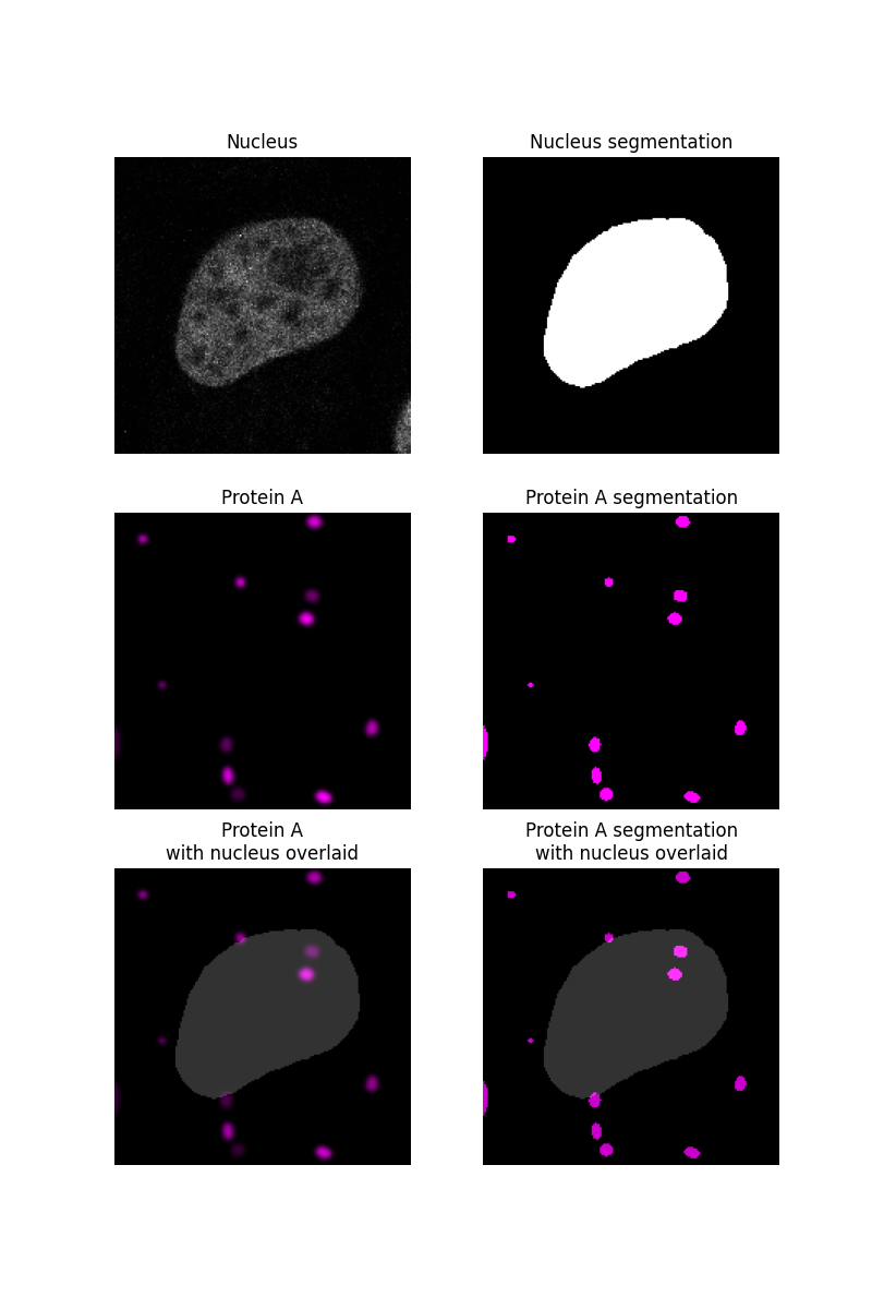
我们首先分割样本图像的细胞核，如另一个 示例中所述，并假设任何不在细胞核中的物质都在细胞质中。蛋白质“蛋白质 A”将被模拟为斑点并分割。

import matplotlib.pyplot as plt
import numpy as np
from matplotlib.colors import LinearSegmentedColormap
from scipy import ndimage as ndi
from skimage import data, filters, measure, segmentation

rng = np.random.default_rng()

# segment nucleus
nucleus = data.protein_transport()[0, 0, :, :180]
smooth = filters.gaussian(nucleus, sigma=1.5)
thresh = smooth > filters.threshold_otsu(smooth)
fill = ndi.binary_fill_holes(thresh)
nucleus_seg = segmentation.clear_border(fill)

# protein blobs of varying intensity
proteinA = np.zeros_like(nucleus, dtype="float64")
proteinA_seg = np.zeros_like(nucleus, dtype="float64")

for blob_seed in range(10):
    blobs = data.binary_blobs(
        180, blob_size_fraction=0.5, volume_fraction=(50 / (180**2)), rng=blob_seed
    )
    blobs_image = filters.gaussian(blobs, sigma=1.5) * rng.integers(50, 256)
    proteinA += blobs_image
    proteinA_seg += blobs

# plot data
fig, ax = plt.subplots(3, 2, figsize=(8, 12), sharey=True)
ax[0, 0].imshow(nucleus, cmap=plt.cm.gray)
ax[0, 0].set_title('Nucleus')

ax[0, 1].imshow(nucleus_seg, cmap=plt.cm.gray)
ax[0, 1].set_title('Nucleus segmentation')

black_magenta = LinearSegmentedColormap.from_list("", ["black", "magenta"])
ax[1, 0].imshow(proteinA, cmap=black_magenta)
ax[1, 0].set_title('Protein A')

ax[1, 1].imshow(proteinA_seg, cmap=black_magenta)
ax[1, 1].set_title('Protein A segmentation')

ax[2, 0].imshow(proteinA, cmap=black_magenta)
ax[2, 0].imshow(nucleus_seg, cmap=plt.cm.gray, alpha=0.2)
ax[2, 0].set_title('Protein A\nwith nucleus overlaid')

ax[2, 1].imshow(proteinA_seg, cmap=black_magenta)
ax[2, 1].imshow(nucleus_seg, cmap=plt.cm.gray, alpha=0.2)
ax[2, 1].set_title('Protein A segmentation\nwith nucleus overlaid')

for a in ax.ravel():
    a.set_axis_off()

交集系数

在分割细胞核和感兴趣的蛋白质后，我们可以确定蛋白质 A 分割有多少部分与细胞核分割重叠。

measure.intersection_coeff(proteinA_seg, nucleus_seg)

0.22

曼德斯共定位系数 (MCC)

重叠系数假设蛋白质分割的面积对应于该蛋白质的浓度 - 较大的面积表示更多的蛋白质。由于图像的分辨率通常太小而无法分辨出单个蛋白质，它们可以在一个像素内聚集在一起，从而使该像素的强度更亮。因此，为了更好地捕获蛋白质浓度，我们可能会选择确定蛋白质通道的强度有多少比例位于细胞核内。此度量称为曼德斯共定位系数。

在此图像中，虽然细胞核内有很多蛋白质 A 点，但它们与细胞核外的一些点相比是暗淡的，因此 MCC 远低于重叠系数。

measure.manders_coloc_coeff(proteinA, nucleus_seg)

np.float64(0.2566709686373243)

在选择共现度量后，我们可以将相同的过程应用于对照图像。如果没有对照图像，可以使用 Costes 方法将原始图像的 MCC 值与随机加扰图像的 MCC 值进行比较。有关此方法的信息在 [1]中给出。

[1]

J. S. Aaron, A. B. Taylor 和 T.-L. Chew，《Image co-localization – co-occurrence versus correlation》，J Cell Sci 2018 年 2 月 1 日 131 (3)：jcs211847。doi：https://doi.org/10.1242/jcs.211847

相关性：两种蛋白质的关联

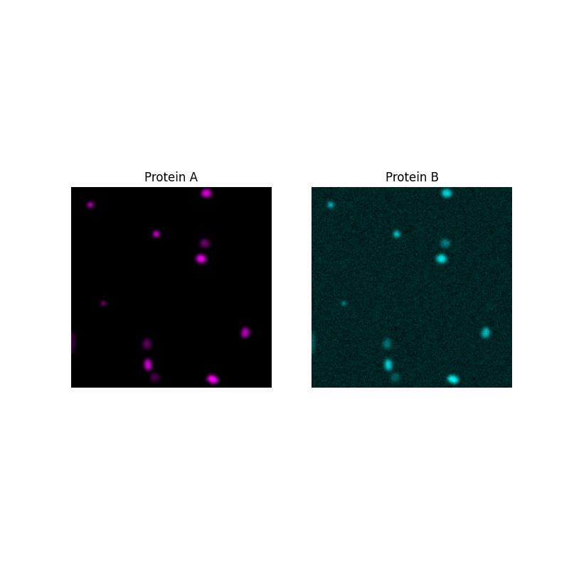
现在，想象一下我们想知道两种蛋白质之间的密切关系。

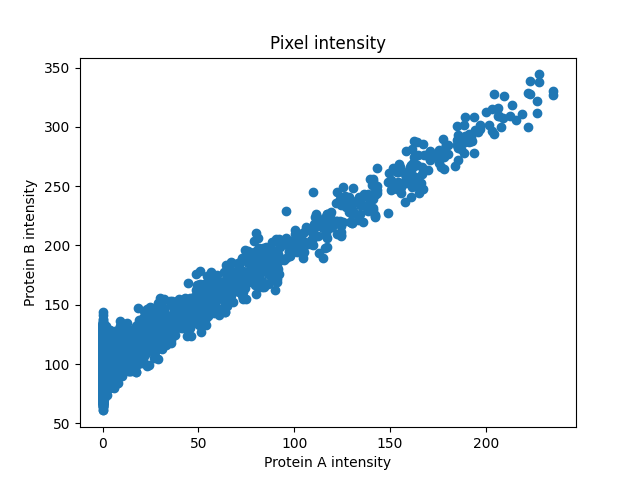
首先，我们将生成蛋白质 B 并绘制每个像素中两种蛋白质的强度，以查看它们之间的关系。

# generating protein B data that is correlated to protein A for demo
proteinB = proteinA + rng.normal(loc=100, scale=10, size=proteinA.shape)

# plot images
fig, ax = plt.subplots(1, 2, figsize=(8, 8), sharey=True)

ax[0].imshow(proteinA, cmap=black_magenta)
ax[0].set_title('Protein A')

black_cyan = LinearSegmentedColormap.from_list("", ["black", "cyan"])
ax[1].imshow(proteinB, cmap=black_cyan)
ax[1].set_title('Protein B')

for a in ax.ravel():
    a.set_axis_off()

# plot pixel intensity scatter
fig, ax = plt.subplots()
ax.scatter(proteinA, proteinB)
ax.set_title('Pixel intensity')
ax.set_xlabel('Protein A intensity')
ax.set_ylabel('Protein B intensity')

• 
• 

Text(38.347222222222214, 0.5, 'Protein B intensity')

强度看起来呈线性相关，因此皮尔逊相关系数可以很好地衡量关联的强度。

pcc, pval = measure.pearson_corr_coeff(proteinA, proteinB)
print(f"PCC: {pcc:0.3g}, p-val: {pval:0.3g}")

PCC: 0.857, p-val: 0

有时，强度是相关的，但不是以线性的方式相关。在这种情况下，像 Spearman 这样的基于秩的相关系数可能会更准确地衡量非线性关系。

plt.show()